Introduction

One of the challenges in remote sensing and working with satellite imagery is how to deal with clouds and shadows. There are various automated routines that exist to aid the researcher such as:

• Using a cloud filter option when downloading the imagery in the first instance.
• Using an automated cloud masking algorithm such as fmask as used by the USGS.

Although these tools are very useful they can be a bit “blunt” as an instrument.

One of the benefits of the explosion of availability of satellite data is that dense temporal analysis can now be performed. Phenological cycles can now be modeled and monitored, for example, and using every suitable image adds more certainty to the analysis. In regions where cloud cover often interferes with data availability it makes sense to be very accurate with with cloud quality assessment.

This workflow has been designed around a “per site” cloud quality assessment protocol. This means that even if an image has been deemed 90% cloud cover, through automated assessment by imagery providers, it still may yield usable data over a site. This method also allows for a more precise identification of:

• Very thin haze associated with smoke.
• Cloud shadows.
• Clouds in bright environment.

Essentially it consists of the following 3 stages which will yield quality assessed time series data for further analysis.

Stage 1. The creation of small jpeg images for each site and date of locally stored satellite data.

Stage 2. Rapid visual assessment of created jpegs with deletion of unsuitable images.

Stage 3. Extraction of data per site for the dates of images that are left after stage 2.

Stage 1

Firstly start by creating a working directory. This must contain a shape file of the sites or locations that ultimately require “clean” data. This directory will become the repository of all the data that is generated through this workflow.

Next task is to run the jpegR function from the RSSApkg.

## Install the RSSApkg if you haven't already
library("devtools")
install_github("RSPaW/RSSApkg")
library("RSSApkg")

## Set up function arguments
# wdir <- path/to/working directory
# imdir <- path/to/imagery directory/pathrow
# layer <- name of shape file that has locations of interest
# attrb <- name of unique id field in shape file
# start <- start image search from this date
# stop <- end image search on this date
# combo <- band numbers to display in RGB
# buffer <- how far to buffer the site location (in metres if imagery is projected to GDA94)

## Run the function
jpegR(wdir, imdir, layer = "my_shape_file", attrb = "siteID", start = "01/12/99", 
      stop = "31-12-2002", combo = c(5,4,2), buffer = 2000)

Things to note about the function arguments:

• wdir and imdir are file paths and need to be character strings.
• layer is a character string of the shape file name without the .shp extension.
• attrb is the field name of the attribute table that stores the unique ID for the locations in the shape file. It is a character string.
• start and end are character strings of dates in either ddmmyy or ddmmY format. It will handle either separator. If you do not provide dates it will search the whole archive. Use these date fields to target your search or to do annual updates and avoid re-processing the entire archive.
• combo are the bands that will be displayed in the red, green and blue channels of the jpeg respectively. In this instance a false colour 542 jpeg will be created. Must be a vector of numbers presented this way.
• buffer for GDA94 projected images the numbers represent meters for the buffer.

The above example would produce jpeg images for each unique location (as designated by id’s found in the ’siteID“” column of the attribute table) in a shape file called “my_shape_file”, for all available satellite data between the dates 01/02/1999 - 31/12/2002. These jpegs would be buffered from the location by 2km and would be a false colour enhancement (542).

For each location a folder will be created in the working directory containing all the jpegs. The folders will be named after the unique locations and will have the naming convention jpegs_site_XXX_bbbbbb_eeeeee where:

• XXX is the unique location id.
• bbbbbb is the first date of imagery processed.
• eeeeee is the last date of imagery processed.

During the process it will also create another folder called site_vectors. At the beginning of the function call, the original shape file contained in the working directory will be split into separate shape files based on the unique locations. These will be stored in this folder along with a small .txt file that contains the name of the original shape file.

Stage 2

Now that the jpegs are created it’s time for a visual assessment. This is not as time consuming or onerous as it sounds. A technique that’s quick is to open up the folder and view the jpegs as “extra large icons”. Then simply delete from the folder any that don’t meet your criteria. The human eye is great at pattern recognition and as soon as the observer becomes familiar with the location, artifacts such as cloud, smoke or haze become easy to spot. Some example images are shown below:

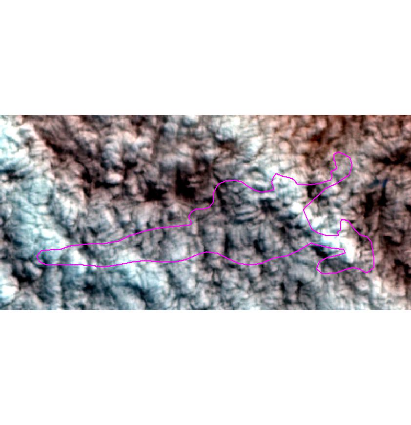
A cloud affected site displayed in false colour 542

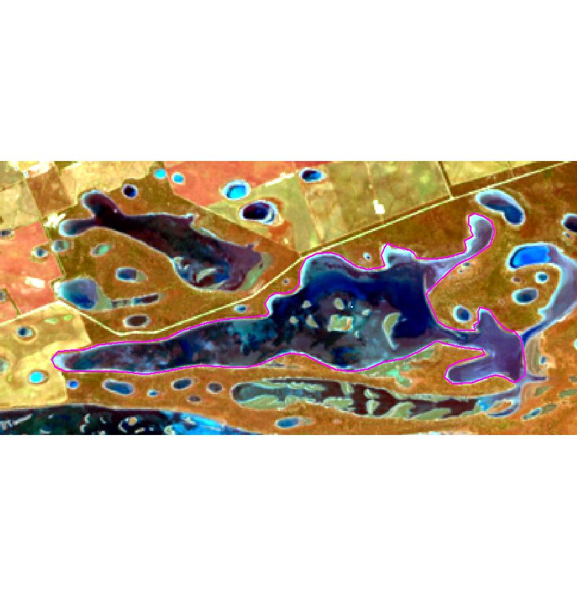
A non-cloud affected site displayed in false colour 542

Not all clouds will be as easy to spot as this example and sometimes shadow can be hard to discern. What can help is re-running jpegR with a larger buffer. This has the effect of “zooming out” and sometimes a broader context can help. The default 2000 is a good starting point.

All the jpegs are named after the date of satellite data that they were created from. By deleting the “bad” jpegs it leaves a folder full of quality assessed dates that will be used in the next stage when values are extracted for each location.

As mentioned the process is quick and an assessor should be able to “QA” as fast as the images are produced.

Stage 3

This last stage entails running the extractR function from the RSSApkg.

## Set up function arguments
# wdir <- path/to/working directory
# imdir <- path/to/imagery directory/pathrow
# option <- band or vegetation index to extract
# attrb <- name of unique id field in shape file

extractR(wdir, imdir, option = "i35", attrb = "siteID")

Things to note about the function arguments:

• wdir and imdir are file paths and need to be character strings.
• option is a character string of one of the following choices. “i35”, “ndvi”, “b1”, “b2”, “b3”, “b4”, “b5” or “b6”. the first 2 are vegetation indices whilst the remaining choices refer to individual bands. Individual band extraction provides the flexibility of producing other indices or band combinations. It must be a character string.
• attrb is the field name of the attribute table that stores the unique ID for the locations in the shape file. It is a character string.

The above example would produce a .csv file containing i35 values for all of the unique locations in the working directory. This file would have the following format. Note NA’s are the results of the quality assessment process removing a particular image date.

..	date	site1	site2	etc
1	10/03/1999	73.11526	NA	etc
2	26/03/1999	37.10274	35.19674	etc
3	14/06/1999	NA	44.44317	etc

This file will have the following naming convention ppprrr_option_QA_bbbbbb-eeeeee.csv where:

• ppprrr is the path/row (6 digits) of the Landsat scene.
• option is what was extracted.
• bbbbbb is the first date of extracted value/s.
• eeeeee is the last date of extracted value/s.

It will also create a separate .csv file per location and store it in the appropriate jpeg folder. These files are formatted slightly differently.

date	site1
10/03/1999	73.11526
26/03/1999	37.10274
etc	etc

These files will have the following naming conventions ppprrr_option_XXX_bbbbbb-eeeeee.csv where:

• ppprrr is the path/row (6 digits) of the Landsat scene.
• option is what was extracted.
• XXX is the unique location id.
• bbbbbb is the first date of extracted value/s.
• eeeeee is the last date of extracted value/s.

NOTE that re-running extractR with the same function arguments will write over the previous output if there have been no new satellite images added to the local archive.

As part of the process, a copy of the unique location shape files, are saved to each of the appropriate jpeg folders. This keeps all of the associated files together for each location.

Updating data sets

It is anticipated that updating the extracted values will be required as new satellite imagery is downloaded and processed (e.g. annual updates). This should be a straight forward process whereby:

• A new working directory is created and the original shape file is copied into it.
• The 3 stages above are followed again but this time restricting jpegR to only the newly acquired image dates.

Any .csv outputs from this update should then be added onto the original outputs.

Need help?

There is a separate vignette for jpegR and extractR which explain some of the finer details. There is also a separate help file written for all functions in the RSSApkg found through the RStudio R Help tab and through the usual R methods if you are not working in RStudio.